日本語は次ページ

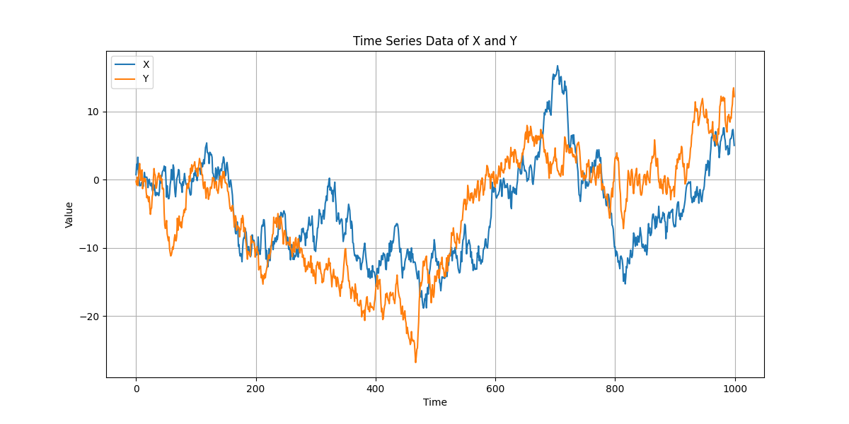
The graph above shows the time series progression of X and Y. It appears that both are moving in tandem.
Based on the assumption that both are correlated, analysts often perform regression analysis, calculate ratios, or take differences between the two.
However, there is an important underlying premise which is that the two are linked.
Revealing the truth: Both are random walk variables
In reality, X and Y are each moving randomly, and there is no actual correlation between them.
Random walk variables literally move randomly, so even if X and Y appear to be moving together, there is no actual correlation between them.
X and Y start at 0 and are generated by sequentially adding 1000 pieces of white noise (uncorrelated, homoscedastic, zero-mean noise). In mathematical terms,
\(X_t = X_{t-1} + \epsilon_t
\)
where 𝜖𝑡 is white noise.
The apparent correlation is purely coincidental, so there is no necessity for their movements to continue being correlated in the future.
This analysis is limited to the artificially generated 1000 pieces of X and Y, but taking the difference between them results in the following pattern.
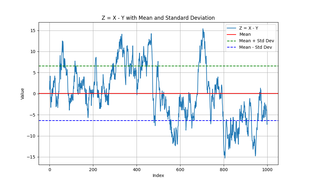
The generated 1000 pieces of X and Y seem to be correlated, so the difference between them (let’s call this Z) should stay within a certain range.
In reality, Z values fall within a certain range (mean ± 1 standard deviation), showing a tendency to revert to the zone when they deviate significantly.
However, to reiterate, since the 1000 pieces of X and Y were randomly generated and only appear to be correlated by chance, there is no guarantee that Z will stay within a certain range in the future.
Important implications from the above
In this case, the variables were randomly generated and only appeared correlated by chance, but if the correlation between X and Y is guaranteed by economic theory, then it can be said that they will continue to be correlated even if they move randomly.
Therefore, it is crucial not to judge solely based on past data, but to validate with data based on theoretical underpinning.
Terminology in Time Series Analysis
The randomly generated variables here are called unit root variables. Since these variables were artificially generated, it is natural that they possess unit roots, but when dealing with economic time series variables, it is unknown whether they have unit roots, so a test called the “unit root test” is performed first.
If multiple time series variables are found to have unit roots, the next step is to test whether they are cointegrated. This is called the “cointegration test,” and if a cointegration relationship is found, it indicates a correlation.
The two random variables used in this article were found to have unit roots via the unit root test (using the ADF test).
Additionally, the cointegration test (using the Engle-Granger test and the Johansen test) also indicated cointegration. The occurrence of “spurious correlation” in the data used this time is rare, and it often fails the cointegration test.
This demonstrates the limitations of statistical hypothesis testing, emphasizing the importance of having a theoretical foundation rather than relying solely on past data.
\ 最新情報をチェック /